Spring Data aggregation operations

MongoDB has a powerful system for aggregating data, called the aggregation pipeline. One particularly useful feature is called bucket operations.

Bucket operations take a collection of documents, and based on a property of those documents, and a list of boundaries, groups those documents into buckets. Each bucket is then transformed into an output document. One output document per bucket.

Buckets are great for time series analysis. Create buckets that break up the time series by day, or by hour, or whatever unit of time, and then perform aggregation operations on the documents within the bucket. For example, find the average temperature by day, the total number of messages sent by hour, or similar type of time series queries.

We are using MongoDB to store images and associated data in a collection called imageCapture. Documents in this collection have many fields, but in this post we’ll focus only on aggregation and consider only two fields on the imageCapture documents:

db.imageCapture.insertMany([
    {
        date: ISODate("2019-11-25T01:13:00.000Z"),
        lbls: ["one", "two", "three"]
    },
    {
        date: ISODate("2019-11-25T04:23:00.000Z"),
        lbls: ["four"]
    },
    {
        date: ISODate("2019-11-26T03:21:00.000Z"),
        lbls: ["five", "six"]
    },
]);

To understand the performance of our system, we want to know how many labels are being detected every day. That is, for every day, we want a sum of the size of the lbls array. This is perfect for MongoDB’s aggregation and bucket capabilities.

Bucket operations in Mongo

To use a bucket operation, we specify the following:

  • groupBy: the field that the boundaries will apply to. This field must be numeric or a date field.
  • boundaries: an array of boundary points. Documents which have a groupBy field falling between two elements in the array go into that bucket. The between test here is half-open, so the first point is inclusive, second point is exclusive, which is the behavior developers would expect
  • default: any documents in the pipeline which don’t go into one of the buckets will go into default. This is required. Using a match operation in the pipeline before the bucket operation will remove documents which shouldn’t be processed.
  • output: an aggregation expression to generate the output document for each bucket

Putting it all together, we create a query as follows:

db.imageCapture.aggregate([
    {
        $bucket: {
            groupBy: "$date",
            boundaries: [ISODate("2019-11-25T00:00:00.000Z"), ISODate("2019-11-26T00:00:00.000Z"), ISODate("2019-11-27T00:00:00.000Z"),
                ISODate("2019-11-28T00:00:00.000Z")],
            default: 'defaultBucket',
            output: {
                "count": {"$sum": {"$size": "$lbls"}}
            }

        }
    }
]);

We have arbitrarily selected some bucket boundaries. The match operation is skipped, but it would be recommended to put a match operation before the bucket in the pipeline, to reduce the number of documents going into the default bucket.

The output could have more fields, too. We might want another field for the most frequently used label in a bucket, or a list of all the labels used in a bucket, for example.

This query works exactly as expected and gives us a count of the total number of labels in each of these buckets. These buckets are not evenly spaced time periods, so this shows that buckets are quite flexible. Buckets are also often used for numeric data. A query might be used to show average income among people in different ranges of credit ratings, for example.

Buckets in Spring Data

Spring Data’s reference guide doesn’t give detailed examples of using buckets. Buckets are such an important feature of MongoDB, it’s worth presenting how to use them in Java. Of course, we could translate the query into a  BasicDBObject, but that’s equivalent to writing SQL query strings and passing them directly to a driver.

Every field in the output is created from an AggregationExpression. In this case, we want an AggregationExpression which is a sum of the size of all the arrays:

final AggregationExpression countingExpression = AccumulatorOperators.Sum.sumOf(ArrayOperators.Size.lengthOfArray("lbls"));

Make a starting point:

        final Instant now = LocalDate.now().atStartOfDay(ZoneOffset.UTC).toInstant();

This starts the time at the start of the day in the UTC timzeone.  Create the BucketOperation with the necessary boundaries, the AggregationExpression, and on the desired field:

final BucketOperation bucketOperation = Aggregation.bucket("date").
                withBoundaries(now.minus(10, ChronoUnit.DAYS), now.minus(9, DAYS),
                        now.minus(8, DAYS), now.minus(7, DAYS), now.minus(6, DAYS),
                        now.minus(5, DAYS), now.minus(4, DAYS), now.minus(3, DAYS),
                        now.minus(2, DAYS), now.minus(1, DAYS), now.minus(0, DAYS)).
                withDefaultBucket("defaultBucket").
                andOutput(countingExpression).as("count");

Now this AggregationOperation can be used in an aggregation pipeline:

final Aggregation aggregation = Aggregation.newAggregation(bucketOperation);

In real use, we would normally want a match operation before the bucket operation in the pipeline. It would be part of the newAggregation call.

Using the aggregation and getting results is very simple. If we had a class that matched the result format we could use that. Otherwise using an implementation of a Map is simple:

final AggregationResults<HashMap> ar = mongoOperations.aggregate(aggregation, "imageCapture", HashMap.class);

The result gives access to a List of HashMaps, accessible by ar.getMappedResults().

Viewing it all together:

        final AggregationExpression countingExpression = AccumulatorOperators.Sum.sumOf(ArrayOperators.Size.lengthOfArray("lbls"));

        final Instant now = LocalDate.now().atStartOfDay(ZoneOffset.UTC).toInstant();

        final BucketOperation bucketOperation = Aggregation.bucket("date").
                withBoundaries(now.minus(10, ChronoUnit.DAYS), now.minus(9, DAYS),
                        now.minus(8, DAYS), now.minus(7, DAYS), now.minus(6, DAYS),
                        now.minus(5, DAYS), now.minus(4, DAYS), now.minus(3, DAYS),
                        now.minus(2, DAYS), now.minus(1, DAYS), now.minus(0, DAYS)).
                withDefaultBucket("defaultBucket").
                andOutput(countingExpression).as("count");
        final Aggregation aggregation = Aggregation.newAggregation(bucketOperation);
        final AggregationResults<HashMap> ar = mongoOperations.aggregate(aggregation, "imageCapture", HashMap.class);
        LOG.info("And the list: " + ar.getMappedResults());

All these classes use a fluent coding style, and we can use static imports, and express it in a more naturally readable style:

        final Instant now = now().atStartOfDay(UTC).toInstant();

        final Aggregation aggregation = newAggregation(bucket("date").
                withBoundaries(now.minus(10, DAYS), now.minus(9, DAYS),
                        now.minus(8, DAYS), now.minus(7, DAYS), now.minus(6, DAYS),
                        now.minus(5, DAYS), now.minus(4, DAYS), now.minus(3, DAYS),
                        now.minus(2, DAYS), now.minus(1, DAYS), now.minus(0, DAYS)).
                withDefaultBucket("defaultBucket").
                andOutput(sumOf(lengthOfArray("lbls"))).as("count"));

        final AggregationResults<HashMap> ar = mongoOperations.aggregate(aggregation, "imageCapture", HashMap.class);

That’s all that’s needed to perform what would be a very complex query in SQL.

Spring Boot CLI

The code for this project is available on GitHub. The project itself runs as a Spring Boot CLI application. This makes it easy to test and experiment with the project. Download from GitHub, enter the project directory, and run:

mvn spring-boot:run

A Survey of Modern AI Physics Modeling

Given a scenario, can an AI model accurately predict the trajectory of moving objects? Can it use knowledge of friction and mass to anticipate the result of objects colliding? These are innate abilities we may take for granted, but attempts to replicate them reveal their complexity.

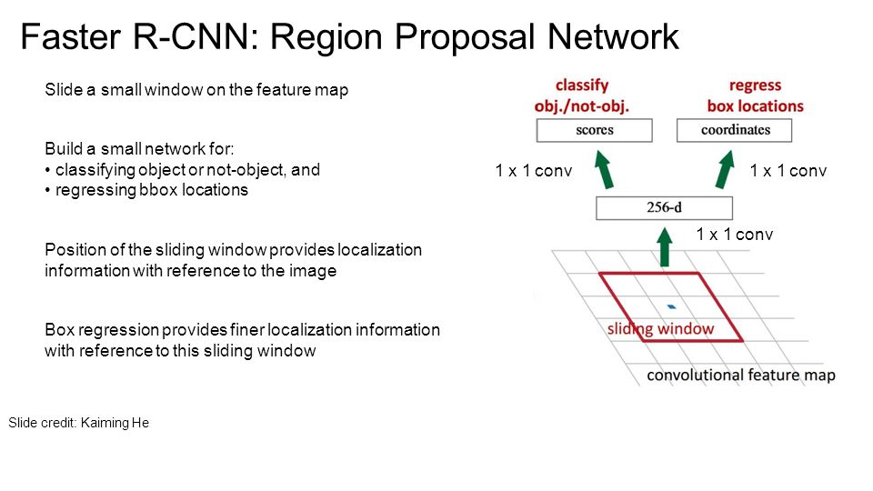
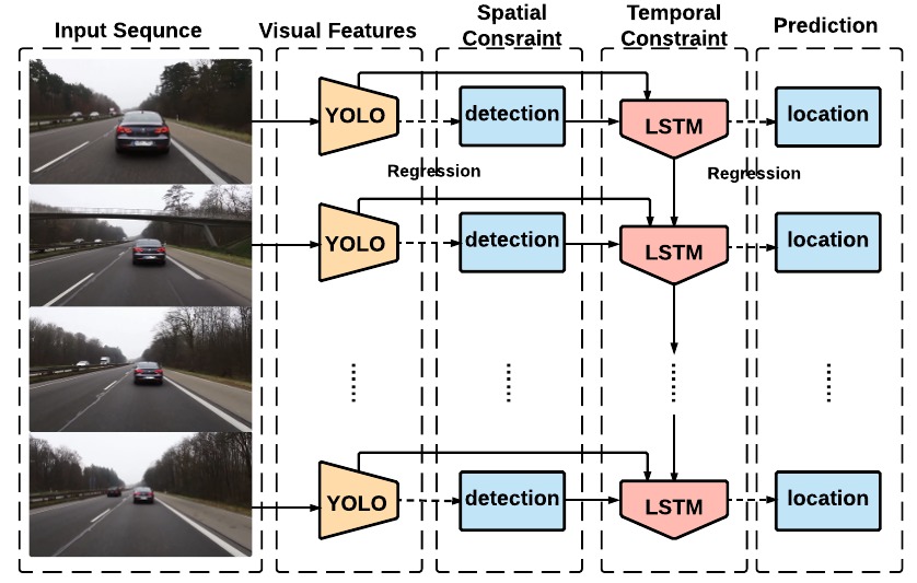
The first project we’ll review isn’t a complete physics system, but it notable for the way it integrates object momentum in a object-detection system. YOLO, short for “You only look once”, is a groundbreaking object-detection system that combines the region proposal and classification steps into one fast regression computation. This system can identify and track objects in real-time. In 2016 PhD student Guanghan Ning released an ingenious modification to YOLO called ROLO. While YOLO would lose track of car moving behind a tree, ROLO could accurately track the car even though it was temporarily obscured by a tree. “Recurrent YOLO for object tracking”, or ROLO, included a long short term memory network, or LSTM. This gave the system a memory of an object’s location and the ability to forecast it. Using the memory, the system learned the speed and momentum of an object, and could estimate it’s position when moving behind an obstacle like a wall, tree, etc. 

ROLO added a temporal dimension to predict trajectory. Source: http://guanghan.info/projects/ROLO/

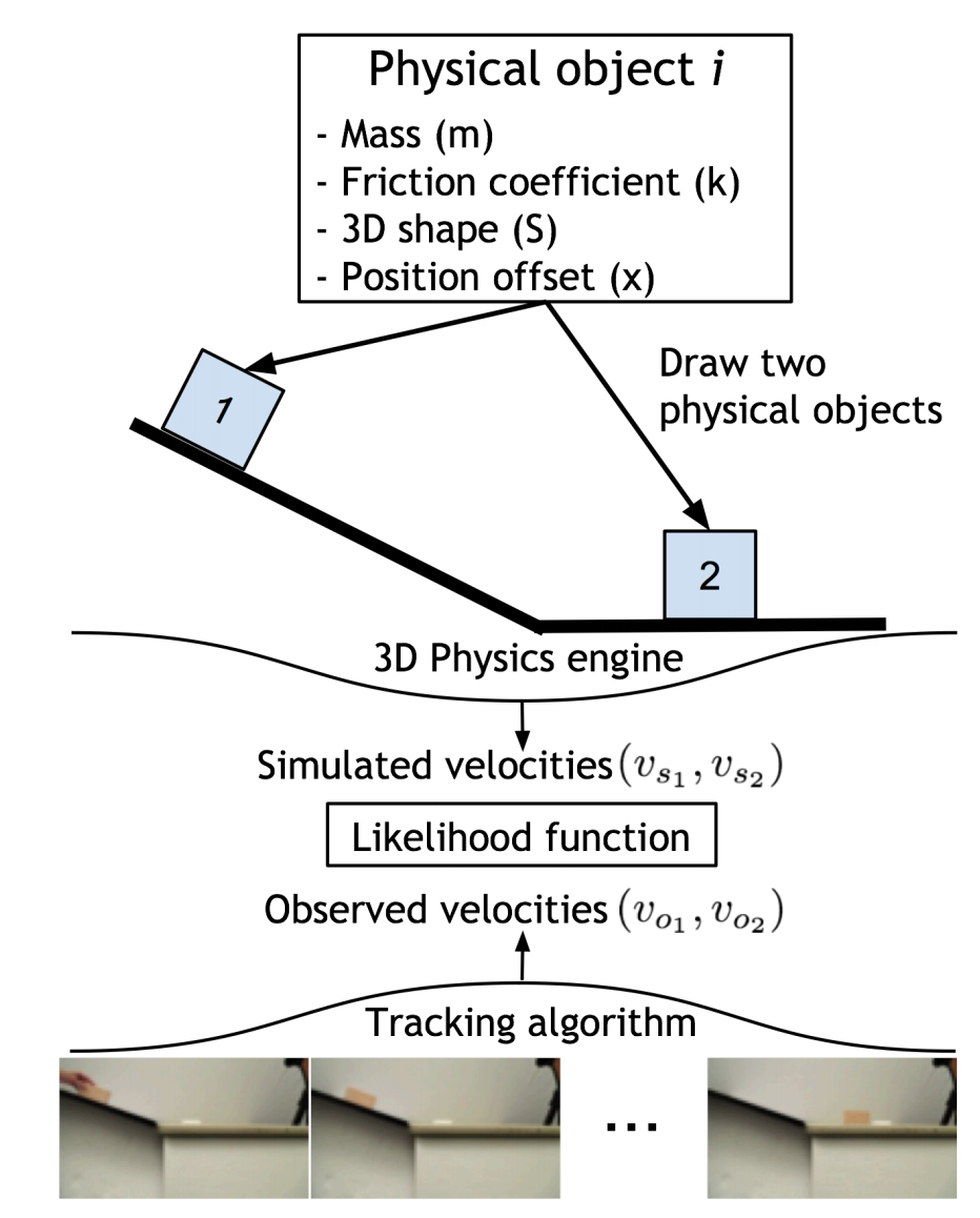
MIT published Galileo in 2015. This system combined deep learning and 3D physics modeling. The researchers set up a simple scenario: an object sliding down an incline and colliding with an object at the bottom. The deep network would estimate physical properties of the two objects. These included mass, friction coefficient, 3D shape, and position. These variables were then applied to a 3D simulation of the same scenario. The 3D physics engine would simulate the sliding and collision of these objects. A tracking algorithm would also calculate the velocity of the real object. With these estimated and recorded inputs, the system simulated and predicted the outcome of the collision. When asked “How far will the object travel after collision?”, humans were accurate 75.3% of the time, while Galileo achieved 71.9% accuracy. Though impressive, this approach requires the physics scenario to be strictly defined.

Galileo uses both 3D simulation and real-world tracking

The next paper attempts to predict physics in a more versatile manner than Galileo. Given an input image and object of focus, the model can automatically infer the correct physics scenario and forecast trajectory. “Newtonian Image Understanding: Unfolding the Dynamics of Objects in Static Images” comes from the Allen Institute for Artificial Intelligence
and the University of Washington. The model consists of two branches. The first is given a video frame with a mask highlighting the object of interest. The second branch is trained on a 3D animation of 12 physics scenarios. Given the input image, the system predicts the correct movement, and then predicts the current state (is the ball already flying though the air or is it at rest?). Though impressive in its versatility, this system is limited to 12 physics scenarios and lacks a thorough internal physics model.

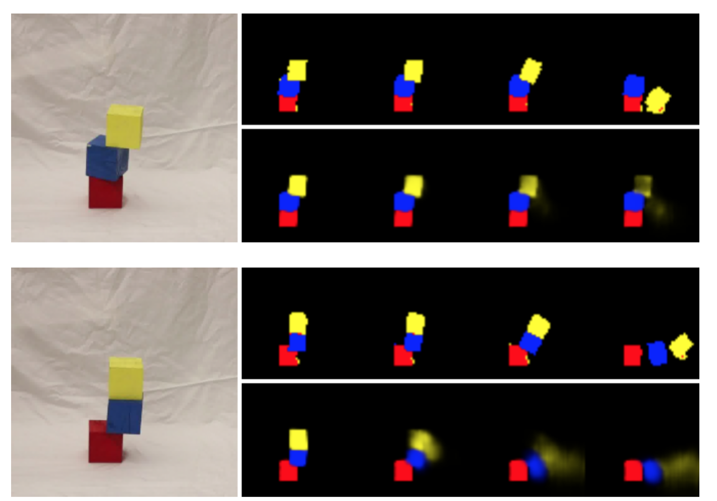
In “Learning Physical Intuition of Block Towers by Example” (2016), Facebook AI Research demonstrated a deep convolutional network that could predict the stability and trajectory of stacked blocks. This approach differs from the above in that it did not leverage 3D modeling for prediction. Instead, this approach relies entirely on deep learning. The models performed well compared to human subjects, and could generalize to unseen scenarios. The figure below shows the model’s results on two scenarios. The figures contain the input image (left), the true outcome (top black background), and the predicted outcome (bottom black background). 

Though an array of modern AI physics systems exist, none achieve the versatility and understanding of human cognition. The approaches may utilize prior physics knowledge in the form of 3D modeling, or they may be fully-deep and infer physics knowledge during training. Both approaches have advantages and disadvantages, and both achieve impressive performance in their test scenarios. 

Relaunched site

We have joined the movement from Drupal to WordPress. We created our own custom theme based on Bootstrap 4. WordPress is easier to edit, especially with the new Gutenberg editor system. Using Bootstrap 4 gives us a responsive site. We used just a few plugins, including support for SVG graphics and relative paths. Overall it’s been an easy change and the site is now much easier to edit, loads faster, looks better, and is responsive.

Some of the old content is being moved over. Most is being deleted, as old technical tips are unhelpful.

Our new site doesn’t work at all on Internet Explorer, due to both the TLS settings, and the use of modern CSS.